Unpacking AlexNet: The Deep Learning Architecture That Changed Everything
In the rapidly evolving world of artificial intelligence, certain milestones stand out as true game-changers. Among them, AlexNet holds a unique and revered position. Winning the ImageNet Large Scale Visual Recognition Challenge (ILSVRC) in 2012, AlexNet didn't just outperform its rivals; it ignited the deep learning revolution, demonstrating the immense power of Convolutional Neural Networks (CNNs) for image recognition at an unprecedented scale.
Prior to AlexNet, traditional computer vision methods struggled with the complexity and variability of real-world images. The model, developed by Alex Krizhevsky, Ilya Sutskever, and Krizhevsky's supervisor Geoffrey Hinton, achieved an astounding top-5 error rate of 15.3%, a significant improvement over the 26.2% of the second-place entry. This wasn't just a win; it was a paradigm shift, proving that deep learning wasn't just a theoretical concept but a practical, high-performing solution.
Let's dive into the technical intricacies of AlexNet and understand the innovations that made it so impactful.
What is AlexNet? A Pioneering CNN
At its core, AlexNet is a deep Convolutional Neural Network designed for image classification. It takes an input image and processes it through a series of convolutional layers, pooling layers, activation functions, and fully connected layers, ultimately outputting a prediction for the image's class (e.g., "cat," "car," "airplane"). Its success was not merely due to its depth, but also to a combination of architectural choices and training techniques that were novel at the time.
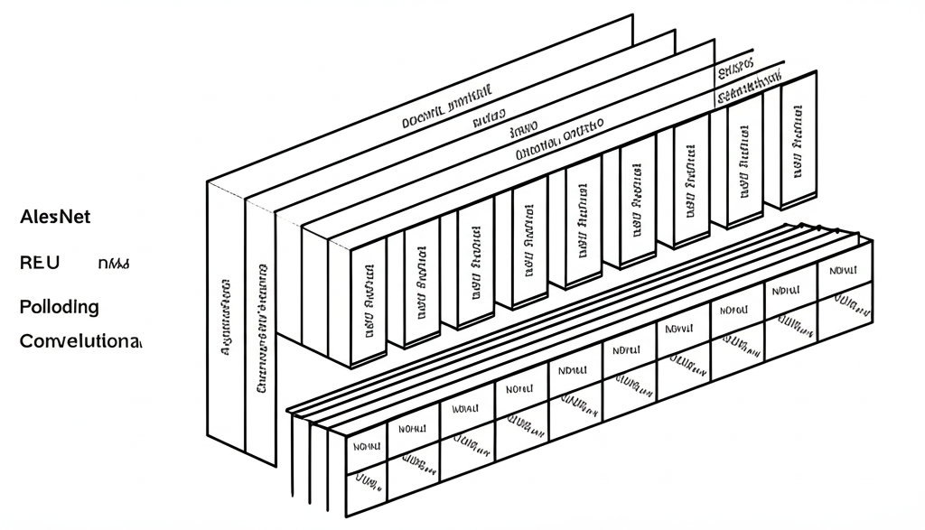
The Architecture Breakdown: Layers and Innovation
AlexNet's architecture consists of eight learned layers: five convolutional layers and three fully connected layers. Let's break down each component:
Input Layer
- The network expects an input image of size 227x227 pixels with 3 color channels (RGB). This specific size was chosen due to the original paper's setup, though often 224x224 is cited due to common practices in subsequent models.
Convolutional Layer 1 (Conv1)
- Filters: 96 filters.
- Filter Size: 11x11.
- Stride: 4 (meaning filters move 4 pixels at a time). This large stride was unusual but helped reduce computation early on.
- Padding: None.
- Activation: Rectified Linear Unit (ReLU).
- Output: 55x55x96 feature maps.
- Followed by Local Response Normalization (LRN) and a 3x3 Max-Pooling layer with a stride of 2. This pooling layer reduces the feature maps to 27x27x96.
Convolutional Layer 2 (Conv2)
- Filters: 256 filters.
- Filter Size: 5x5.
- Padding: 2 (to maintain spatial dimensions).
- Activation: ReLU.
- Output: 27x27x256.
- Also followed by LRN and a 3x3 Max-Pooling layer with a stride of 2, reducing feature maps to 13x13x256.
Convolutional Layer 3 (Conv3)
- Filters: 384 filters.
- Filter Size: 3x3.
- Padding: 1.
- Activation: ReLU.
- Output: 13x13x384.
Convolutional Layer 4 (Conv4)
- Filters: 384 filters.
- Filter Size: 3x3.
- Padding: 1.
- Activation: ReLU.
- Output: 13x13x384.
Convolutional Layer 5 (Conv5)
- Filters: 256 filters.
- Filter Size: 3x3.
- Padding: 1.
- Activation: ReLU.
- Output: 13x13x256.
- Followed by a 3x3 Max-Pooling layer with a stride of 2, reducing feature maps to 6x6x256.
Fully Connected Layer 6 (FC6)
- The output from the last pooling layer (6x6x256) is flattened into a 1D vector of 9216 features (66256).
- Neurons: 4096.
- Activation: ReLU.
- Regularization: Dropout (probability 0.5).
Fully Connected Layer 7 (FC7)
- Neurons: 4096.
- Activation: ReLU.
- Regularization: Dropout (probability 0.5).
Output Layer (FC8)
- Neurons: 1000 (corresponding to the 1000 classes of the ImageNet dataset).
- Activation: Softmax, which produces a probability distribution over the 1000 classes.
Key Innovations That Powered AlexNet's Success
AlexNet wasn't just a deep network; it was a cleverly designed one that integrated several crucial innovations, some of which are still cornerstones of deep learning today:
1. ReLU (Rectified Linear Unit) Activation Function
- What it is: Instead of traditional activation functions like sigmoid or tanh, AlexNet used ReLU, defined as
f(x) = max(0, x). - Why it mattered: ReLUs significantly accelerate training convergence compared to saturating nonlinearities. They help mitigate the vanishing gradient problem, allowing deeper networks to be trained effectively.
2. Dropout Regularization
- What it is: During training, dropout randomly sets a fraction of the output of neurons to zero at each update.
- Why it mattered: This technique prevents complex co-adaptations between neurons, effectively forcing the network to learn more robust features. It acts as a powerful regularization method, preventing overfitting, especially in large networks like AlexNet with millions of parameters.
3. Local Response Normalization (LRN)
- What it is: Inspired by lateral inhibition in real neurons, LRN normalizes activations across feature maps. It makes features more salient by enhancing the contrast of the active neurons.
- Why it mattered: While effective for AlexNet, LRN is rarely used in modern CNNs, having been largely superseded by techniques like Batch Normalization, which offer superior performance and stability.
4. Extensive Data Augmentation
- What it is: To prevent overfitting and increase the effective size of the training dataset, AlexNet used various data augmentation techniques.
- Why it mattered: This included random cropping (227x227 patches from 256x256 images), horizontal flipping, and varying the intensity of RGB channels (PCA-based augmentation). These transformations made the network more robust to variations in input images.
5. GPU Implementation
- What it is: AlexNet was one of the first deep learning models to heavily leverage Graphics Processing Units (GPUs) for training. The network was split across two GPUs to fit within their memory constraints.
- Why it mattered: Training such a large and deep network on the massive ImageNet dataset would have been prohibitively slow on CPUs. GPUs provided the parallel processing power necessary to train the model in a reasonable timeframe (5-6 days).
Training Details
- Dataset: ImageNet Large Scale Visual Recognition Challenge (ILSVRC-2010), containing 1.2 million high-resolution images across 1000 different classes.
- Optimizer: Stochastic Gradient Descent (SGD) with momentum.
- Learning Rate: Started at 0.01 and was decreased manually when the validation error stopped improving.
- Weight Decay: L2 regularization was used to further prevent overfitting.
The Enduring Legacy of AlexNet
AlexNet's victory in 2012 was a pivotal moment, unequivocally demonstrating that deep CNNs could learn incredibly powerful and hierarchical features directly from raw image data, surpassing traditional feature engineering methods. It paved the way for an explosion of research and development in deep learning, leading to increasingly sophisticated architectures like VGG, ResNet, Inception, and many more.
Its principles—deep layers, ReLU activations, dropout regularization, and GPU acceleration—became foundational elements for future deep learning models. AlexNet didn't just win a competition; it opened the floodgates for the era of modern AI, inspiring countless researchers and engineers to explore the vast potential of neural networks in computer vision and beyond.